Lab 7

Due Thursday March 5 at 11:59 PM

Let \(X\) be a random variable, let \(g\) be a transformation, and consider the new random variable \(Y=g(X)\). If all we cared about was the mean of \(Y\), then LOTUS provides a nice shortcut for computing \(E(Y)=E[g(X)]\) directly. But often, we want to know the entire distribution of the new random variable \(Y\), not just the mean. Today we will learn how to calculate it.

The template

In all that follows, \(X\) is continuous with pdf \(f_X\) and cdf \(F_X\). The goal in each case is to compute the density \(f_Y\) of the new random variable \(Y=g(X)\). The process for doing this is always the same:

Plot the transformation \(g\) so you understand what’s going on;
Figure out what \(\text{Range}(Y)\) is;
Find the cdf of \(Y\): \(F_Y(y)=P(Y\leq y)\);
Differentiate it to get the pdf: \(f_Y(y)=F'_Y(y)\).

This is the so-called “cdf method.”

Task 0 (watch the TA)

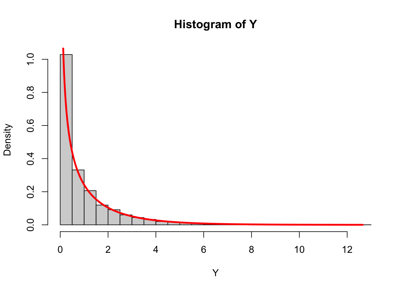
If \(Z \sim \text{N}(0, 1)\), what is the pdf of \(Y = Z^{2}\)? Turns out it’s a member of the gamma family! See below for the derivation.

Derivation

We know that \(\text{Range}(Z)=\mathbb{R}\) and that

\[ \begin{aligned} f_Z(z)&=\frac{1}{\sqrt{2\pi}}e^{-z^2/2},&&z\in\mathbb{R}\\ F_Z(z)&=\frac{1}{\sqrt{2\pi}}\int_{-\infty}^ze^{-t^2/2}\,\text{d}t,&&z\in\mathbb{R}. \end{aligned} \]

Newsflash: the cdf of the normal distribution is unknown. We can approximate it arbitrarily well using numerical methods, but we don’t actually have a clean formula for it. The integral above is simply intractable.

The transformations involved here are the quadratic and (principal) square root functions. Note the following:

neither the quadratic nor the square root can be applied to negative numbers
when applied to nonnegative numbers, both the quadratic and square root give nonnegative numbers back
when applied to nonnegative numbers, both functions are strictly-increasing or order-preserving
the quadratic function is even (i.e., \(x^{2} = (-x)^{2}\))

All of these facts will help us in this derivation. First, we know that the quadratic function is nonnegative, so we see then that \(\text{Range}(Y)=[0,\,\infty)\). Fixing \(y\geq 0\), we compute:

\[ \begin{align*} F_Y(y)&=P(Y\leq y)\\ &=P(Z^2\leq y)\\ &=P\left(-\sqrt{y}\leq Z\leq \sqrt{y}\right)\\ &=F_Z\left(\sqrt{y}\right) - F_Z\left(-\sqrt{y}\right). \end{align*} \]

As such, the pdf is:

\[ \begin{aligned} f_Y(y) = F'_Y(y)&=\frac{\text{d}}{\text{d} y}F_Z\left(\sqrt{y}\right) - \frac{\text{d}}{\text{d} y}F_Z\left(-\sqrt{y}\right)\\ &=F_Z'\left(\sqrt{y}\right)\frac{\text{d}}{\text{d}y}\left[\sqrt{y}\right] - F_Z'\left(\sqrt{y}\right)\frac{\text{d}}{\text{d}y}\left[-\sqrt{y}\right]\\ &=f_Z\left(\sqrt{y}\right)\frac{1}{2\sqrt{y}} - f_{Z}\left(-\sqrt{y}\right)\left(-\frac{1}{2\sqrt{y}}\right)\\ &=\frac{1}{2\sqrt{y}}\left(f_{Z}\left(\sqrt{y}\right) + f_{Z}\left(-\sqrt{y}\right)\right)\\ &=\frac{1}{2\sqrt{y}}\left(f_{Z}\left(\sqrt{y}\right) + f_{Z}\left(\sqrt{y}\right)\right)&&\text{(standard normal pdf is even function)}\\ &=\frac{1}{2\sqrt{y}}\left(2 \cdot f_{Z}\left(\sqrt{y}\right)\right)\\ &=\frac{1}{\sqrt{y}}f_{Z}\left(\sqrt{y}\right)\\ &=\frac{1}{\sqrt{y}}\frac{1}{\sqrt{2\pi}}e^{-\left(\sqrt{y}\right)^{2}/2}\\ &=\frac{1}{\sqrt{2\pi}}y^{-1/2}e^{-y/2},&&y\geq 0. \end{aligned} \]

At first blush, this may not look particularly gamma-ish. However, using a variant of “massaging and squinting,” we can reveal the gamma.

Recall that, for a \(Y \sim \text{Gamma}(\alpha, \beta)\) random variable, the pdf is of the form \[ f_{Y}(y) = \frac{\beta^{\alpha}}{\Gamma(\alpha)}y^{\alpha - 1}e^{-\beta y}, \quad y \geq 0. \] Our massaging and squinting will involve rewriting (1) the exponent of \(y\) and (2) the normalizing constant \(\frac{\beta^{\alpha}}{\Gamma(\alpha)}\). Using a result that you will prove in problem set 5, we then have the following:

\[ \begin{aligned} f_{Y}(y)&=\frac{1}{\sqrt{2\pi}}y^{-1/2}e^{-y/2}\\ &=\frac{1}{\sqrt{2}} \cdot \frac{1}{\sqrt{\pi}}y^{1/2 - 1}e^{-y/2}\\ &=\left(\frac{1}{2}\right)^{1/2} \cdot \frac{1}{\Gamma\left(\frac{1}{2}\right)}y^{1/2 - 1}e^{-y/2}\\ &=\frac{(1/2)^{1/2}}{\Gamma\left(\frac{1}{2}\right)}y^{1/2 - 1}e^{-y/2},&&y \geq 0. \end{aligned} \] So, \(Y \sim \text{Gamma}\left(\frac{1}{2}, \frac{1}{2}\right)\).

This matches with a simulation:

set.seed(20)
Z <- rnorm(5000)
Y <- Z^2
hist(Y, breaks = "Scott", freq = FALSE)
curve(dgamma(x, shape = 0.5, rate = 0.5), from = min(Y), to = max(Y), n = 1000, 
      col = "red", lwd = 3, add = TRUE)

In particular, the distribution we derived here is a member of a subfamily of the gamma distribution family known as the chi-squared distribution.

Task 1

Consider \(X\sim \text{Gamma}(1,\,1)\). This is the same as saying \(X\sim\text{Exponential}(1)\), which we saw in lecture on Monday.

What are the range and pdf of \(Y=\ln X\)?
Simulate n = 5000 draws of \(Y\). Plot a histogram, and add a line plot of the density you derived in part b. They should match!

Solution

To begin, we know that \(\text{Range}(X)=[0,\,\infty)\) and

\[ \begin{aligned} F_X(x)&=1-e^{-x},&&x\geq0\\ f_X(x) &= e^{-x}, &&x\geq0. \end{aligned} \]

One of our math helpers displays the graph of the natural log and its inverse, the exponential. Consulting these, we note a few things:

the natural log takes in strictly positive numbers and spits out both positive and negative numbers;
both the natural log and the exponential are strictly increasing. In other words, they are order-preserving.

The first property implies that \(\text{Range}(Y)=\mathbb{R}\). So fix arbitrary \(y\in \mathbb{R}\). The cdf of \(Y\) is

\[ \begin{aligned} F_Y(y)&=P(Y\leq y)\\ &=P(\ln X\leq y)\\ &=P(e^{\ln X}\leq e^y)\\ &=P\left(X\leq e^y\right)\\ &=F_X\left(e^y\right)\\ &=1-e^{-e^y}. \end{aligned} \]

Since the exponential function is order-preserving, we didn’t have to chage the inequality when we applied it to both sides. To get the pdf, take a derivative (using the chain rule!):

\[ f_Y(y)=F_Y'(y)=\frac{\text{d}}{\text{d} y}\left(1-e^{-e^y}\right)=0-(-e^y)e^{-e^y}=e^{y-e^y},\quad y\in\mathbb{R}. \]

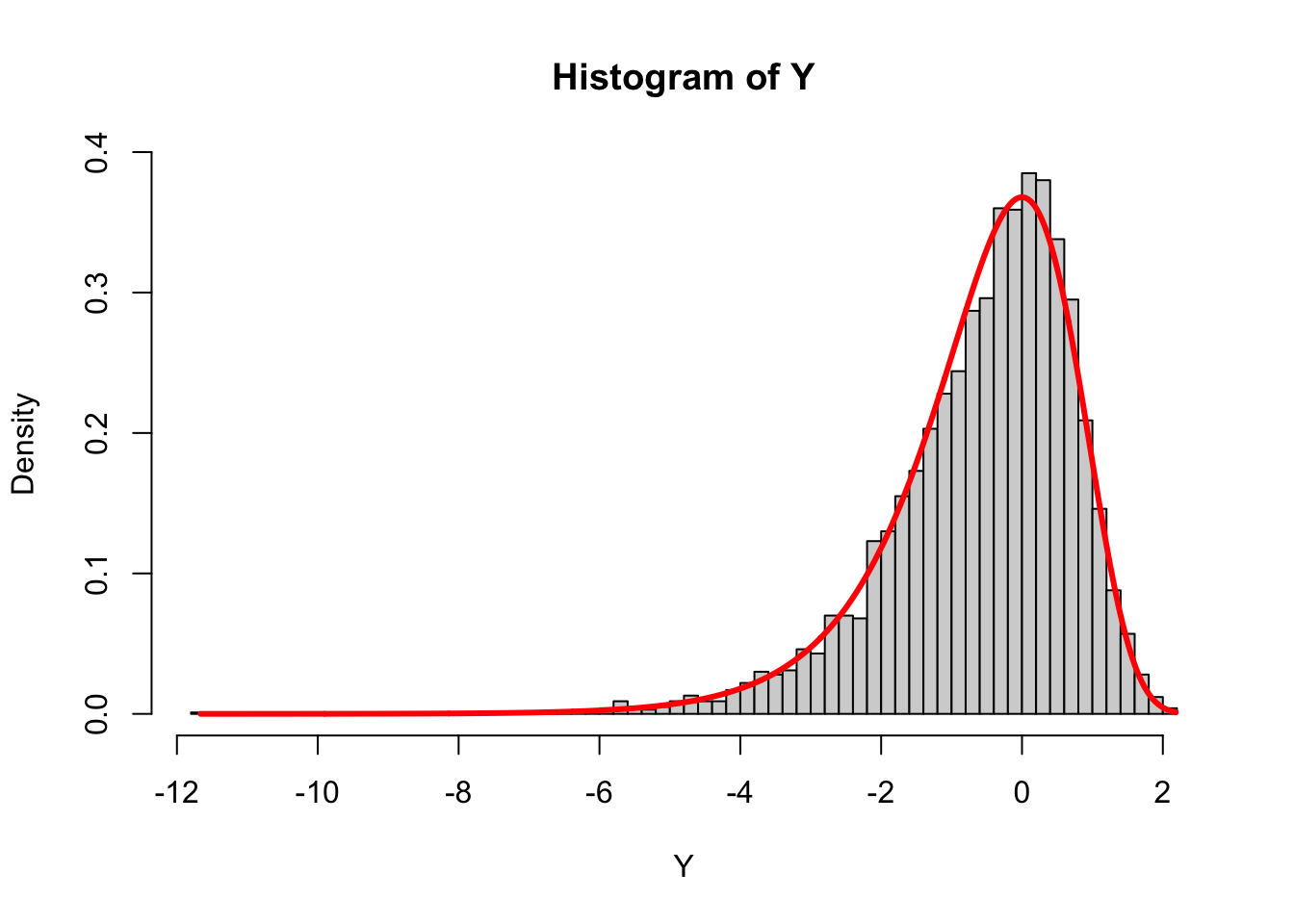
If we compare this density to the histogram from a simulation, they agree:

set.seed(20)
X <- rgamma(5000, shape = 1, rate = 1)
Y <- log(X)
hist(Y, breaks = "Scott", freq = FALSE)
curve(exp(x - exp(x)), from = min(Y), to = max(Y), n = 1000, 
      col = "red", lwd = 3, add = TRUE)

Phew!

Task 2

Consider \(X\sim\text{Unif}(-\pi/2,\,\pi/2)\).

What are the range and pdf of \(Y=\tan X\)?
Simulate n = 5000 draws of \(Y\). Plot a histogram, and add a line plot of the density you derived in part b. Can you get them to match?

Solution

By construction, \(\text{Range}(X)=(-\pi/2,\,\pi/2)\). You can read more about the continuous uniform here, and we see see that the cdf is

\[ F_X(x) = \begin{cases} 0 & x\leq -\frac{\pi}{2}\\ \frac{x-\left(-\frac{\pi}{2}\right)}{\frac{\pi}{2}-\left(-\frac{\pi}{2}\right)} & -\frac{\pi}{2}<x<\frac{\pi}{2}\\ 1 & \frac{\pi}{2}\leq x. \end{cases} \]

So when \(-\frac{\pi}{2}<x<\frac{\pi}{2}\), we have

\[ F_X(x)=\frac{x+\frac{\pi}{2}}{\pi}=\frac{x}{\pi}+\frac{1}{2}. \]

The transformation is

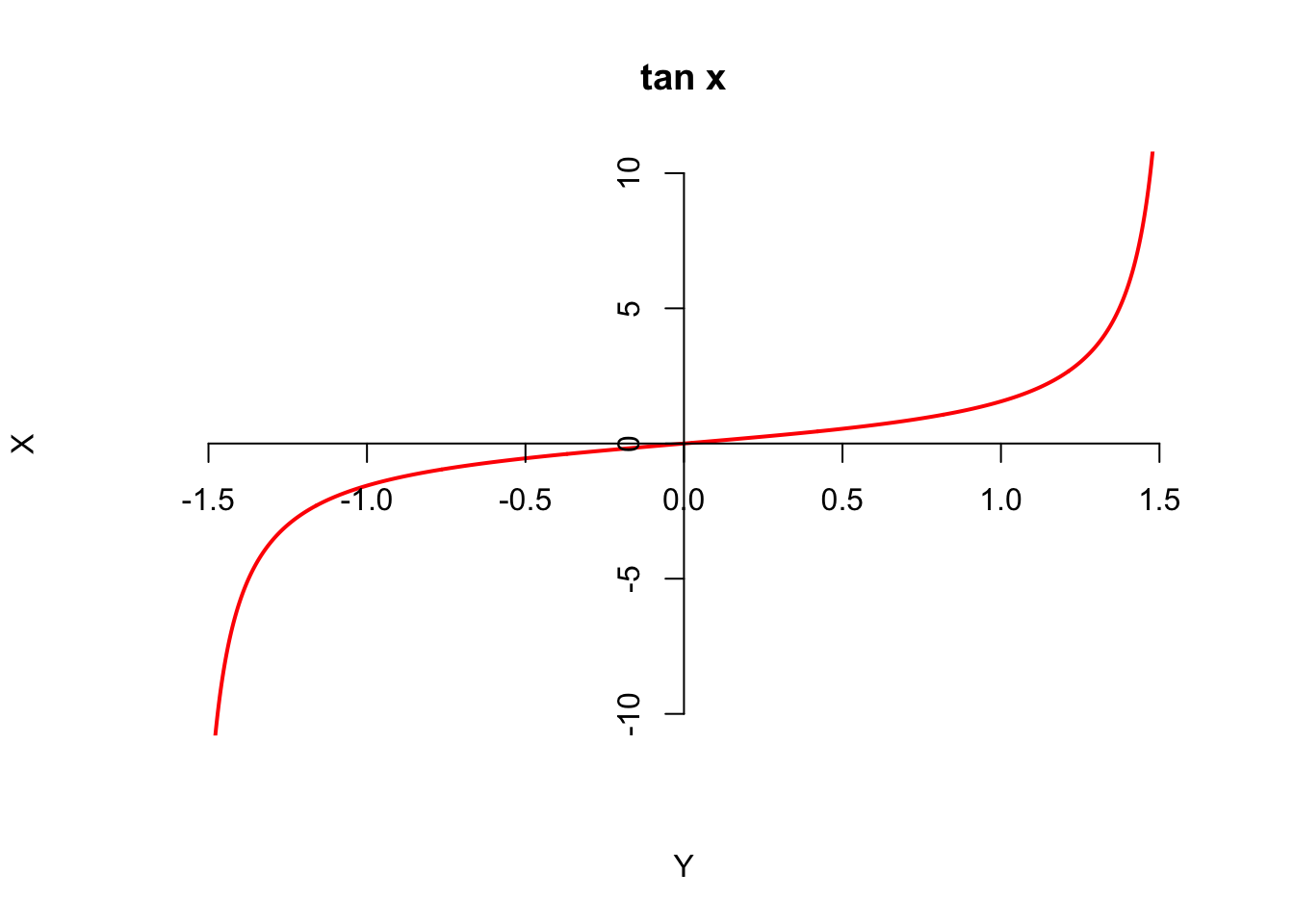
Again, strictly-increasing, and it maps to all real numbers. So \(\text{Range}(Y)=\mathbb{R}\). Now let’s fix arbitrary \(y\in\mathbb{R}\) and find the cdf:

\[ \begin{aligned} F_Y(y)&=P(Y\leq y)\\ &=P(\tan X\leq y)\\ &=P(X\leq \tan^{-1}y)\\ &=F_X(\tan^{-1}y)\\ &=\frac{\tan^{-1}y}{\pi}+\frac{1}{2}. \end{aligned} \]

Take a derivative to get the pdf:

\[ f_Y(y) = F'_Y(y) = \frac{\textrm{d}}{\textrm{d}y} \left( \frac{\tan^{-1}y}{\pi}+\frac{1}{2} \right) = \frac{1}{\pi(1+y^2)},\quad y\in\mathbb{R}. \]

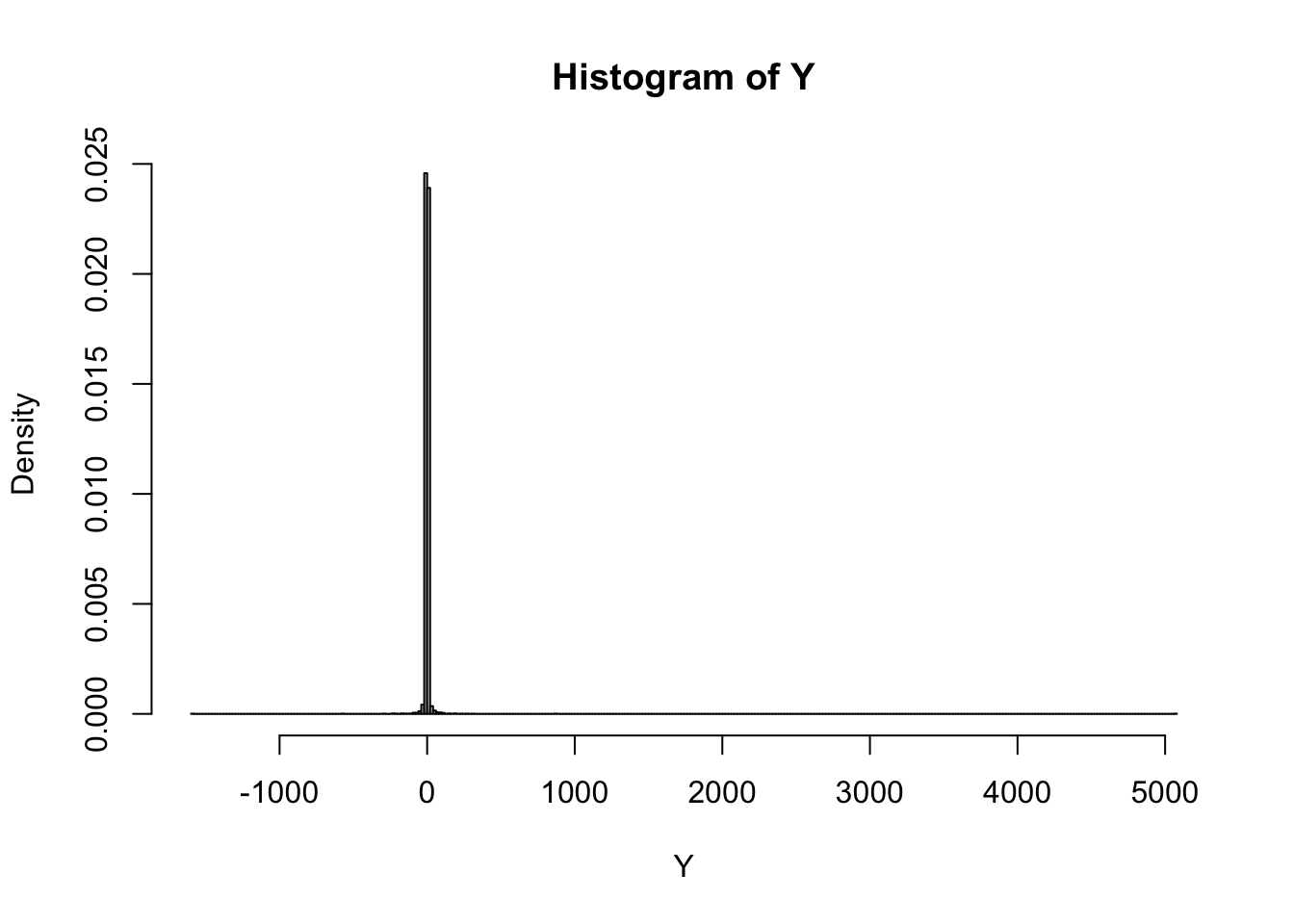
Rest assured that we did the math right, but you’d have a hard time verifying it with a simulation:

set.seed(20)
X <- runif(5000, -pi / 2, pi / 2)
Y <- tan(X)
hist(Y, breaks = "Scott", freq = FALSE)

Here is the graph of the density we derived, and for reference I added the pdf of the standard normal distribution (bell curve):

Code

curve(dnorm(x), from = -7, to = 7, n = 1000, ylab = "", bty = "n")
curve(dcauchy(x), from = -7, to = 7, n = 1000, add = TRUE, col = "red")
legend("topright", c("N(0, 1) density", "Cauchy density"), bty = "n",
       lty = 1, col = c("black", "red"))

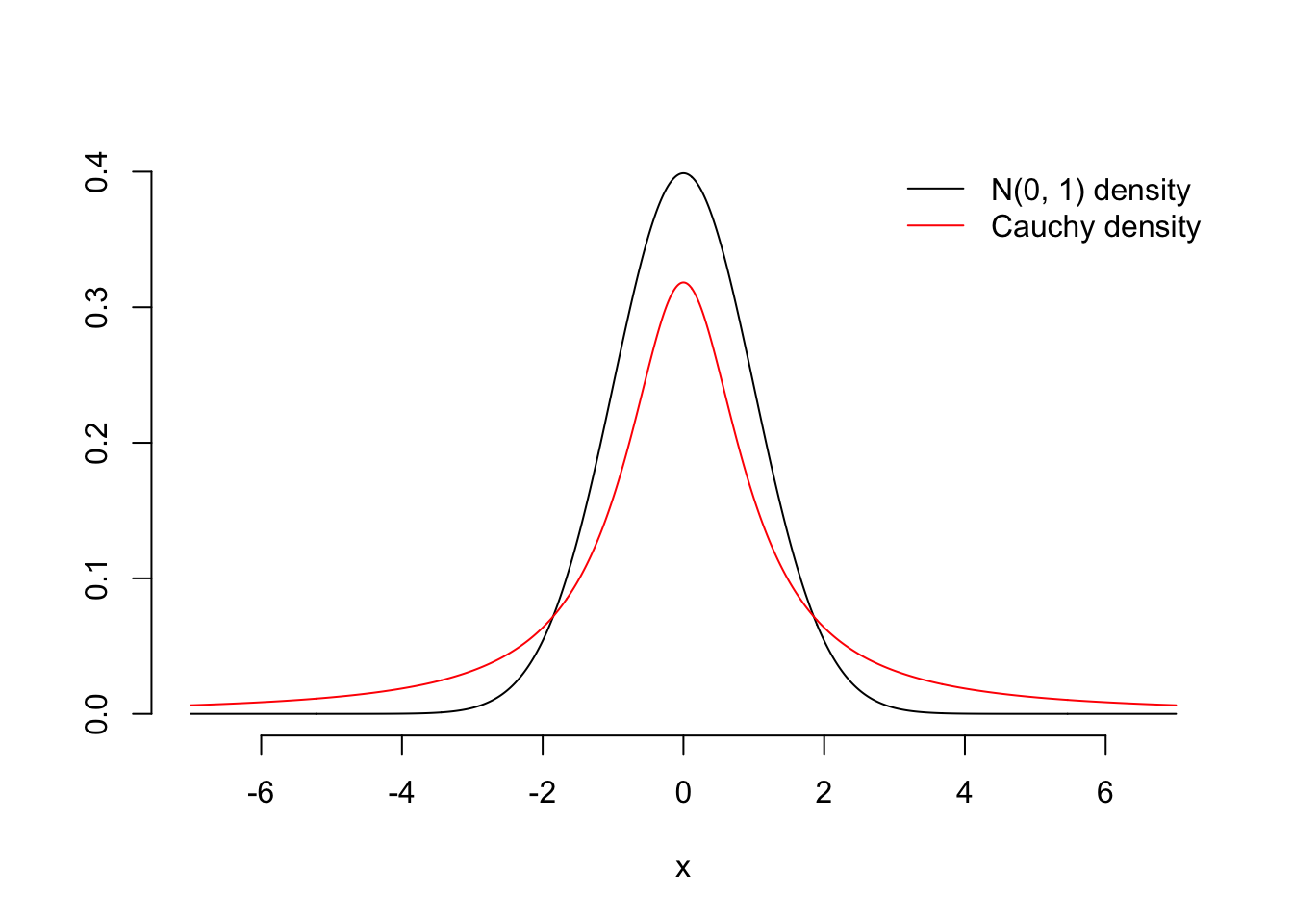
Compared to the bell curve, this new density has very heavy tails. They are so heavy in fact that this distribution does not have a finite mean or variance or any other moment. It is very ill-behaved, and it frequently surprises with extreme values far out in the tails. That’s why the histogram looks awful and always will.

This distribution we just derived is quite famous. It’s called the Cauchy distribution.

Task 3

Consider \(X\sim \text{N}(0,\,1)\).

What are the range and pdf of \(Y=e^X\)?
Simulate n = 5000 draws of \(Y\). Plot a histogram, and add a line plot of the density you derived in part b. They should match!

Solution

We know that \(\text{Range}(X)=\mathbb{R}\) and that

\[ \begin{aligned} f_X(x)&=\frac{1}{\sqrt{2\pi}}e^{-x^2/2},&&x\in\mathbb{R}\\ F_X(x)&=\frac{1}{\sqrt{2\pi}}\int_{-\infty}^xe^{-t^2/2}\,\text{d}t,&&x\in\mathbb{R}. \end{aligned} \]

Anyway, the transformations involved here are again the exponential and the natural log, which we already saw in Task 1. Both are strictly-increasing. The exponential takes any real number and maps it to something strictly positive, so we see then that \(\text{Range}(Y)=(0,\,\infty)\). Fixing \(y>0\), we compute:

\[ \begin{align*} F_Y(y)&=P(Y\leq y)\\ &=P(e^X\leq y)\\ &=P\left(X\leq \ln y\right)\\ &=F_X\left(\ln y\right). \end{align*} \]

As such, the pdf is:

\[ \begin{aligned} f_Y(y) = F'_Y(y)&=\frac{\text{d}}{\text{d} y}F_X(\ln y)\\ &=F_X'(\ln y)\frac{\text{d}}{\text{d}y}\ln y\\ &=f_X(\ln y)\frac{1}{y}\\ &=\frac{1}{\sqrt{2\pi}}e^{-(\ln y)^2/2}\frac{1}{y},&&y>0. \end{aligned} \]

This matches with a simulation:

set.seed(20)
X <- rnorm(5000)
Y <- exp(X)
hist(Y, breaks = "Scott", freq = FALSE)
curve(dnorm(log(x)) / x, from = min(Y), to = max(Y), n = 1000, 
      col = "red", lwd = 3, add = TRUE)

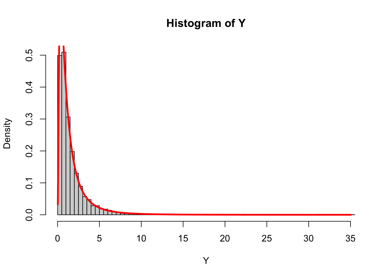
The distribution we derived here is an example of the log-normal distribution.

Interlude

Given \(X\sim f_X\), we want the density of \(Y=g(X)\). In the three examples, you followed the same basic steps:

write the generic cdf of \(Y\): \(F_Y(y)=P(Y\leq y)=P(g(X)\leq y)\);
rewrite the event inside until \(X\) is by itself (you probably have to undo or invert \(g\) to do this);
since \(X\) is by itself, rewrite the probability using the cdf of \(X\);
differentiate (you probably have to use the chain rule to do this).

The basic template can be neatly summarized with the so-called change-of-variables formula, which tells you how to compute the density of \(Y\) using the density of \(X\) and the transformation \(g\):

\[ f_Y(y)=f_X\left(g^{-1}(y)\right) \left|\frac{\text{d}}{\text{d} y}g^{-1}(y)\right|,\quad y\in\text{Range}(Y). \]

Proof

Assume…

\(X\) is absolutely continuous with pdf \(f_X\);
\(g\) is defined for all \(x\in\text{Range}(X)\);
\(g\) is differentiable and either strictly increasing or strictly decreasing (hence, invertible).

There are two cases:

Strictly increasing

If \(g\) is strictly increasing, then \(g^{-1}\) is strictly increasing also. This means that \(\frac{\text{d}}{\text{d} y}g^{-1}(y)\) must be positive for all \(y\)! It also means that \(g^{-1}\) is order-preserving. If \(a\leq b\), then \(g^{-1}(a)\leq g^{-1}(b)\).

Fix arbitrary \(y\in\text{Range}(Y)\). Then:

\[ \begin{aligned} F_Y(y) &= P(Y\leq y) \\ &= P\left(g(X)\leq y\right) \\ &= P\left(X\leq g^{-1}(y)\right) \\ &= F_X\left(g^{-1}(y)\right) . \end{aligned} \]

Taking a derivative and applying the chain rule gives

\[ \begin{aligned} f_Y(y) &= \frac{\text{d}}{\text{d} y}F_X\left(g^{-1}(y)\right) \\ &= f_X\left(g^{-1}(y)\right)\underbrace{\frac{\text{d}}{\text{d} y}g^{-1}(y)}_{\text{positive!}} \\ &= f_X\left(g^{-1}(y)\right) \left|\frac{\text{d}}{\text{d} y}g^{-1}(y)\right|. \end{aligned} \]

Strictly decreasing

If \(g\) is strictly decreasing, then \(g^{-1}\) is strictly decreasing also. This means that \(\frac{\text{d}}{\text{d} y}g^{-1}(y)\) must be negative for all \(y\)! It also means that \(g^{-1}\) is order-reversing. If \(a\leq b\), then \(g^{-1}(a)\geq g^{-1}(b)\).

Fix arbitrary \(y\in\text{Range}(Y)\). Then:

\[ \begin{aligned} F_Y(y) &= P(Y\leq y) \\ &= P\left(g(X)\leq y\right) \\ &= P\left(X> g^{-1}(y)\right) \\ &= 1-P\left(X\leq g^{-1}(y)\right) \\ &= 1-F_X\left(g^{-1}(y)\right) . \end{aligned} \] Taking a derivative and applying the chain rule gives

\[ \begin{align*} f_Y(y) &= \frac{\text{d}}{\text{d} y}[1-F_X\left(g^{-1}(y)\right)] \\ &= {\color{red}-}f_X\left(g^{-1}(y)\right)\underbrace{\frac{\text{d}}{\text{d} y}g^{-1}(y)}_{\text{negative!}} \\ &= f_X\left(g^{-1}(y)\right) \left|\frac{\text{d}}{\text{d} y}g^{-1}(y)\right|. \end{align*} \]

Either way, we got to the same place.

Task 4

Let \(X\) be an absolutely continuous random variable with pdf \(f_X\), let \(a,\,b\in\mathbb{R}\) be non-zero constants, and consider the new random variable \(Y=aX+b\).

What is \(E(Y)\)?
What is \(\text{var}(Y)\)?
Use the change-of-variables formula to find the density of \(Y\)?
In the special case where \(X\sim\text{N}(0,\,1)\), what are \(E(Y)\), \(\text{var}(Y)\), and the density of \(Y\)? There’s no need to re-derive anything here. Just plug what you know about N(0, 1) into the formulas from parts a, b, and c.

Sanity check

When you do part (d), you should see that a linear transformation of a normal IS ITSELF normal. (Note: This is not true for every distribution family.)

Solution

We know from lecture that \(E(Y)=E(aX+b)=aE(X)+b\) and \(\text{var}(Y)=\text{var}(aX+b)=a^2\text{var}(X)\).

If \(g(x)=ax+b\) is the linear transformation, then the inverse transformation and its derivative are

\[ \begin{align*} g^{-1}(y)&=\frac{y-b}{a}\\ \frac{\text{d}}{\text{d} y}g^{-1}(y)&=\frac{1}{a}, \end{align*} \]

and the change-of-variables formula gives:

\[ f_Y(y)=f_X\left(\frac{y-b}{a}\right)\frac{1}{|a|}. \]

If \(X\sim\text{N}(0,\,1)\), then we know from lecture that \(E(X)=0\), \(\text{var}(X)=1\), and

\[ f_X(x)=\frac{1}{\sqrt{2\pi}}\exp\left(-\frac{1}{2}x^2\right),\quad x\in\mathbb{R}. \]

A new random variable \(Y=aX+b\) has

\[ E(Y)=aE(X)+b=a\cdot 0+b=b, \]

and

\[ \text{var}(Y)=a^2\text{var}(X)=a^2\cdot 1=a^2, \]

and

\[ f_Y(y)=\frac{1}{|a|}\frac{1}{\sqrt{2\pi}}\exp\left(-\frac{1}{2}\left(\frac{x-b}{a}\right)^2\right)=\frac{1}{\sqrt{2\pi a^2}}\exp\left(-\frac{1}{2}\frac{\left(x-b\right)^2}{a^2}\right). \]

So \(Y\sim \text{N}(b,\, a^2)\). That’s where the general normal comes from: you apply a linear transformation to the standard normal.