Lab 8

Due Thursday March 19 at 11:59 PM

When we call rnorm or rgamma or rpois to generate random numbers from one of our special distributions, what is the computer actually doing? How do we program a computer to generate random numbers that behave according to some pre-defined distribution?

At the end of the day, all simulation methods revolve around a simple principle: “simulate from the standard uniform and then apply a transformation.” We statisticians take from granted that the computer scientists have devised good methods for generating random numbers from Unif(0, 1). The Mersenne Twister is a popular algorithm. Given that we can generate random numbers from the standard uniform, we need to figure out how to transform them into a batch of new random numbers that follow the distribution we want: normal, gamma, Cauchy, whatever.

Task 0

The following theorem is a proof of concept that “simulate Unif(0, 1) and transform” is sufficient, at least in theory, to simulate any distribution we can think of:

Theorem: inverse transform sampling

Let \(U\sim \text{Unif}(0,\, 1)\), and let \(F\) be any continuous cdf we are interested in. If we define a new random variable \(X=F^{-1}(U)\), then \(X\sim F\).

Proof

For simplicity, assume \(F\) is smooth and invertible. Things still work if it isn’t, but it makes the math a little cleaner. Furthermore, recall the cdf of the standard uniform \(U\sim\text{Unif}(0,\, 1)\): \[ F_U(x)=\begin{cases} 0 & x \leq 0\\ x & 0<x<1\\ 1 & 1 \leq x. \end{cases} \]

\(X\) is just a transformation of \(U\), so we can apply the cdf method. \[ \begin{align*} F_X(x) &= P(X\leq x) \\ &= P(F^{-1}(U)\leq x) \\ &= P(U\leq F(x)) \\ &= F_U\left(F(x)\right) \\ &= F(x) . \end{align*} \]

So, the cdf of \(X\) is literally just \(F\).

Now, in order to actually implement the algorithm, we need to be able to compute the inverse cdf \(F^{-1}\). In some cases, this may not be possible, and we must use a different transformation to actually get the job done. But the principle stands. Dig down deep enough into any simulation algorithm, and it’s just simulating uniforms and messing with them.

Task 1 (you do it)

Consider a random variable \(X\) with this density:

\[ f(x) = \frac{e^{-x}}{(1+e^{-x})^2},\quad x\in\mathbb{R}. \]

Compute the cdf;
Compute the inverse cdf;
Use inverse transform sampling to generate n = 5000 random numbers from this distribution. Plot a histogram of the random numbers, and overlay a line plot of the original density function we gave you. If you did everything correctly, the histogram and the density should agree.

Task 2 (you do it)

Consider a random variable \(X\) with this density:

\[ f(x) = xe^{-\frac{1}{2}x^2},\quad x\geq 0. \]

Compute the cdf;
Compute the inverse cdf;
Use inverse transform sampling to generate n = 5000 random numbers from this distribution. Plot a histogram of the random numbers, and overlay a line plot of the original density function we gave you. If you did everything correctly, the histogram and the density should agree.

Task 3 (we do it)

Consider a random variable \(X\) with this density:

\[ f(x) = e^{-(x+e^{-x})},\quad x\in\mathbb{R}. \]

Compute the cdf;
Compute the inverse cdf;
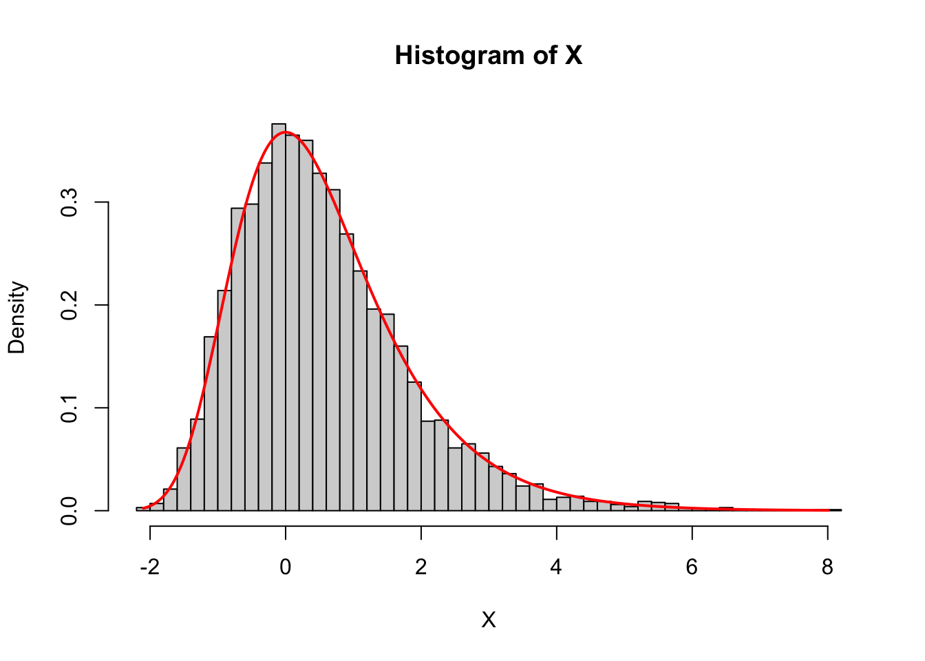
Use inverse transform sampling to generate n = 5000 random numbers from this distribution. Plot a histogram of the random numbers, and overlay a line plot of the original density function we gave you. If you did everything correctly, the histogram and the density should agree.

Solution

This is the standard Gumbel distribution.

\[ \begin{aligned} F(x) &= \int_{-\infty}^x f(t) dt \\ &= \int_{-\infty}^x e^{-(t+e^{-t})} dt \\ &= \int_{\infty}^{e^{-x}} -e^{-(-\ln u+u)} \frac{du}{u} && \begin{matrix} u=e^{-t}\\ du=-e^{-t}\,dt \end{matrix} \\ &= \int_{e^{-x}}^\infty e^{-u}du \\ &= [-e^{-u}]_{e^{-x}}^\infty \\ &= 0-(-e^{-e^{-x}}) \\ &= e^{-e^{-x}},&& x\in\mathbb{R}. \end{aligned} \]

Invert it:

\[ \begin{aligned} u &= e^{-e^{-x}}\\ \ln u&=-e^{-x}\\ -\ln u &=e^{-x}\\ \ln(-\ln u)&=-x\\ -\ln(-\ln u)&=x. \end{aligned} \]

\[ F^{-1}(u)=-\ln(-\ln u),\quad 0<u<1. \]

set.seed(152638)
U <- runif(5000)
X <- -log(-log(U))
hist(X, breaks = "Scott", freq = FALSE)
curve(exp(-x-exp(-x)), from = min(X), to = max(X), n = 1000, 
      col = "red", lwd = 2, add = TRUE)

Task 4 (we do it)

Consider a random variable \(X\) with this density:

\[ f(x) = \frac{1}{2}e^{-|x|},\quad x\in\mathbb{R}. \]

Compute the cdf;
Compute the inverse cdf;
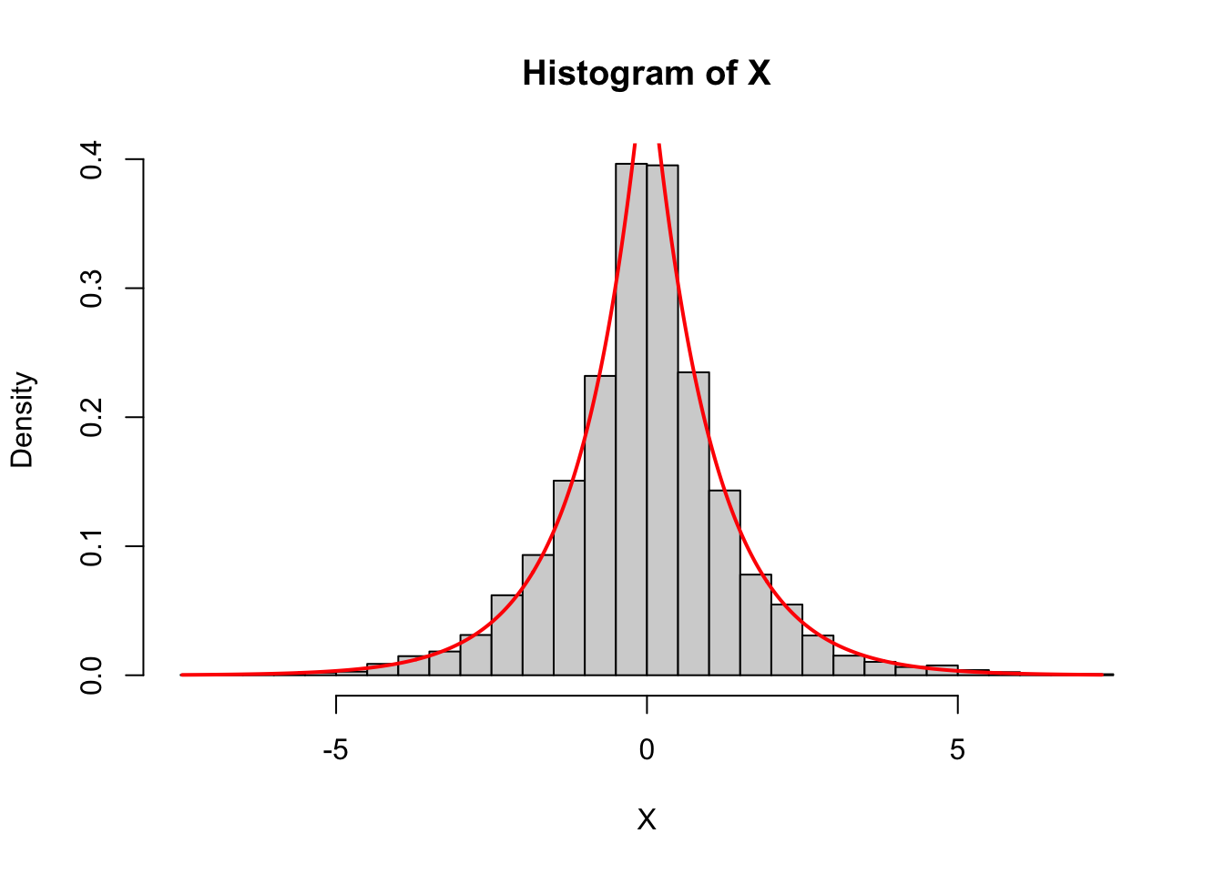
Use inverse transform sampling to generate n = 5000 random numbers from this distribution. Plot a histogram of the random numbers, and overlay a line plot of the original density function we gave you. If you did everything correctly, the histogram and the density should agree.

Solution

This is the standard Laplace distribution. For \(x<0\),

\[ \begin{aligned} F(x) &= \int_{-\infty}^x \frac{1}{2}e^{-|t|}\,\text{d}t \\ &= \frac{1}{2} \int_{-\infty}^x e^{-(-t)}\,\text{d}t \\ &= \frac{1}{2} \int_{-\infty}^x e^{t}\,\text{d}t \\ &= \frac{1}{2} [e^t]_{-\infty}^x \\ &= \frac{1}{2} e^x. \end{aligned} \]

For \(x\geq 0\),

\[ \begin{aligned} F(x)&=P(X\leq x) \\ &=1-P(X>x) \\ &=1-\int_x^\infty \frac{1}{2}e^{-|t|}\,\text{d}t \\ &= 1-\frac{1}{2}\int_x^\infty e^{-t}\,\text{d}t \\ &= 1-\frac{1}{2}[-e^{-t}]_x^\infty \\ &= 1-\frac{1}{2}e^{-x}. \end{aligned} \]

\[ \begin{aligned} F(x) &= \begin{cases} \frac{1}{2} e^x & x<0\\ 1-\frac{1}{2} e^{-x} & x\geq 0. \end{cases} \end{aligned} \]

If you invert that darn thing, you get:

\[ \begin{aligned} F^{-1}(u)=\text{sign}(0.5 - u)\ln(1-2|u-0.5|),\quad 0<u<1. \end{aligned} \]

set.seed(152638)
U <- runif(5000)
X <- sign(0.5 - U) * log(1 - 2 * abs(U - 0.5))
hist(X, breaks = "Scott", freq = FALSE)
curve(0.5 * exp(-abs(x)), from = min(X), to = max(X), n = 1000, 
      col = "red", lwd = 2, add = TRUE)

Task 0

Task 1 (you do it)

Task 2 (you do it)

Task 3 (we do it)

Task 4 (we do it)

Further reading